A year ago, I found an online hint about typing a name for a chart in a cell, then linking to it. It only worked about half the time, and I could never figure out why. Today I finally solved the mystery of the linked chart title, and I want to share my discovery.
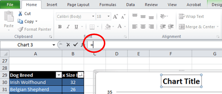
 Click on the title of the chart. Press the function key on your keyboard labeled “F2” or simply click your cursor on the Formula Bar.
This is the shortcut for editing any cell – now you are editing your chart title. Your cursor will jump up to the Formula Bar. Type = and click on your cell reference. When you hit enter, your title will match your cell.
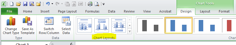
Just in case you have a chart without a title, click on the edge of your chart. The Chart Tools menu will appear. In the Chart Layout section, select a layout with a title – the ones with a bluish box near the top. You can click the down arrow to get more selections.