How to explain the difference between using a relative and absolute cell reference in a basic Excel formula? I know that most people get nervous around any math, but how about a multiplication table? Do children still learn that in third grade like I did. I still know that 12×12=144! When writing a complicated formula in Excel, I will often start with small numbers that I know, so let’s use a multiplication table to learn about relative and absolute cell references.
I will also offer some quick lessons on about Excel’s “fill” commands, Paste Transpose, and Paste Formula to speed things along.
I use the Verdana font whenever I am working with numbers. It was created specifically to help you see the differences between numbers like “6” and “8.”
Autofill and the Autofill Cursor

In Cell A1, type a big “X” to show that we are multiplying. (Is this reminding you of second or third grade now?)
In Cell A2, Enter the number “1.” In Cell A3, Enter the number “2.“ With those two cell entries, Excel will know that you are counting when you use Autofill.Select Cells A2 and A3 by dragging through both.

Hover your mouse over the bottom right corner of your range. A small “+” will appear called the “Fill” cursor. Pull the fill cursor down. Excel will continue counting and show you how far you have gotten with the numbers in the small square right of your cursor. Stop when you get to “12.” When you let go of the mouse button, Excel will ‘fill” those cells with numbers 1 to 12.

Copy and Paste Transpose
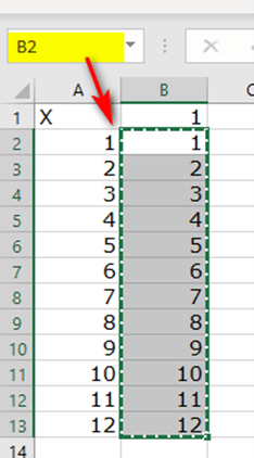
Drag through Cells A2:A12, so that our numbers 1 to 12 are selected. Right-click Copy to copy this to the Excel Clipboard. A green dotted marquee outline will appear. Click on Cell B1, just to the right of our “X.” Now right-click and look at the paste options. Hover your mouse over the one with paste clipboard with the two arrows: one pointing down and one pointing right.
This is the Paste Transpose option. It takes a vertical range and makes it horizontal. Or it can take a horizontal range and make it vertical. As you hover your mouse over it, you will see our numbers 1 to 12 appear across the top of the spreadsheet. Click that Paste Transpose clipboard. Using Paste Transpose, you copied and pasted our numbers 1 to 12 across the top of the spreadsheet.
Multiplication Formula

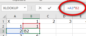
In Cell B2, enter the formula to multiply “1×1.” Always start a formula with an equals sign (=). Now click on Cell A2 to place our cell reference in to the formula. Type an asterisk (*) to tell Excel to multiply. (Excel thinks “x” is a letter, but an asterisk is the operand to multiply in Excel language.) Click on Cell B1 to finish the formula. Press Enter to enter the formula into Excel.
Excel Copy & Paste: Fill Right, Fill Down and AutoFill
By selecting two consecutive cells A2:A3 with consecutive numbers 1 and 2, we used Autofill to fill in numbers from 1 to 12. By just selecting one cell to start, rather than a range, you can use Autofill as a shortcut for copy and paste. You can also use Fill Down or Fill Right (or Up or Left) command. Select Cell B2 with our multiplication formula. Drag down to Cell B13, so that the Range B2:B3 is highlight. From the Home), from Home tab>Editing section>Fill drop-down arrow, select Fill Down. Similar to Autofill, our formula is copied and pasted into all the cells from B2 to B13.

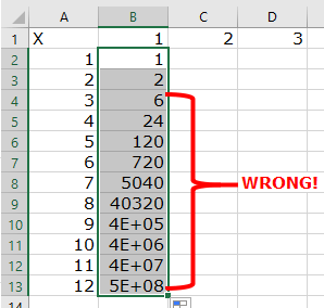
Oops! If you know your “ones” times tables, you will see that there was a BIG problem.
Formula References with Copy & Paste
You will see some very large numbers appearing in Column B that do not look like a multiplication table. Those relative references did not work Click on Cell B3 and click in the Formula Bar to see what went wrong! When you moved down one cell to paste, your Cell references also moved down one.
Moving your references one by one is great in some situations. Say you have columns for each month. If you are calculating sales quotas, you want the same formula in each column as you move from January to February to March, right? That is how Excel copies and pastes by default. If you copy a formula three cells right and two cells down, then all the formula references will be three cells right and two cells down. That is how “Relative” references work.
Show Formulas
From the Formulas tab>Formula Auditing section>select Show Formulas. Excel spreads out the column width. Instead of showing the value inside the cell, Excel shows us the actual formulas within each cell. Cell B1 shows us “=A2*B1 with the color-coding. You can click through any cell and see the color-coding.
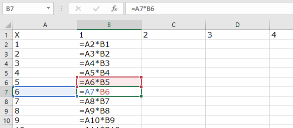
Click on Cell B7. In a Multiplication Table, Cell B7 should be multiplying the number 6 In Cell A7 by the number 1 in Cell B1 at the top of Column B. Instead it is shifted down and is multiplying A7 times B6…. So our numbers are wrong and just keep getting bigger and more wrong! Show Formulas is a toggle switch. Press once to turn it on and again to turn it off. Leave it on for now.
Relative & Absolute References
When Excel copied our formulas down, it changed all the cell references down. It Is multiplying the number one cell left times the number one cell above. Excel is always guessing what we want. Usually when we move or paste something to the right, the formulas change one to the right. When we move down one cell, it move all the cell references down to the next cells.
This is called a “Relative” reference, and “relative” is Excel’s default mode.
When you want to pinpoint a specific column, row, or cell, you want that reference to be “Absolute.” You need to always tell Excel when you want an “Absolute” reference. Turn off “Show Formulas” by clicking it again.
As we copy and paste new information into our cells, it will delete was there and put in the new information. You may also delete the incorrect information before we try again or use Ctrl-Z to undo our Fill Down. (I will use Ctrl-Z.) I like working with our multiplication tables, because we know if they are right or wrong with a glance, right?

Using F4 or “$” for Absolute
Click on Cell B2. In the Formula Bar, click between the first cell reference, A2 – in other words, click between the “A” and the “2” on the Formula Bar. You should see your cursor flashing right there.
Back in the “old” days with early spreadsheet software or “apps,” Visicalc and Lotus 123 were designed to be used without a mouse. We used the Function Keys at the top of the keyboard to get around. F5 is/was “go to.” F2 is/was edit. F4 is all about absolute references.
Press F4. Excel will put two dollar signs “$” in your cell reference: $A$2. Each dollar sign means “DO NOT CHANGE WHEN COPYING!” So do not change from Column A and do not change from Row 2.

Press F4 again. Excel takes one dollar sign “$” away: A$2. This means you can change from Column A, but do not change from Row 2.
Guess what happens if you press F4 again. Do it. Now you have $A2. (Do not change from Column A.)
Press F4 again to go back to the original “relative” cell reference of A2.
Go through the whole sequence again, seeing it change: $A$2, A$2, $A2, A2. Stop on $A2.
You may have seen these dollar signs before. When we set up a range for the Print Area or Print Titles, Excel puts the dollar signs, aka, absolute references, in for us.
Multiplying with Column A and Row 1
For our Multiplication Table, we want to multiply by the left-hand Column A and the top Row 1. Those are the absolute references that should not change.
Look at the Formula Bar for Cell B2. You always want to use the numbers in Column A to multiply.
So in the first cell reference, A2, press F4 until it says $A2. That means the Column A will always be part of the equation. We want the cell reference to continue moving down, row by row in Column A.

Now click on the second cell reference in the Formula Bar, “B1.” We want to always use the numbers in Row 1 for our multiplication. Press F4 until you have B$1. This tells Excel to always use Row 1.
Press Enter or the checkmark in the Formula Bar to enter our new formula. (You may have noticed Excel is putting ideas in the Cell Address box, such as “XLOOKUP.” Ignore those.)
The multiplication is still working for Cell B2: 1×1=1. Now try Fill Down or AutoFill to copy and paste our formula to Range B3:B13. It worked in Column B.
Paste Formula
You may use AutoFill or Fill Right to complete our Multiplication Table, but there is one more Paste option you should know. If you want to paste a formula without any of is formatting, you can use Copy and Paste Formula.
Drag through Cell B2 to B13 (also written Range B2:B13). Home tab>Copy (or Ctrl-C or right-click Copy). The green dotted marquee will be there. Be sure you are not including Row 1, and that B2 is showing the Formula Bar’s Address Box.
Now select the range to copy your formula with the corrected “absolute” factors from Cell C2 to Cell M2… one cell under numbers 2 through 12.
From the Home tab>Clipboard section>select the Paste drop-down arrow. (You may right-click Paste.) DO NOT use Ctrl-V.
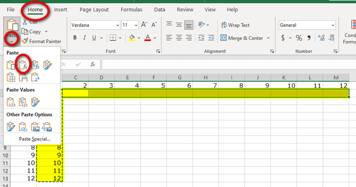
The Paste Formula (only) clipboard is the clipboard with the function symbol “fx.” Click the Paste Formula clipboard.
Go through your times tables in your head. Are all the numbers correct?
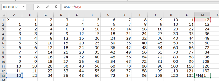
Click on Cell M12 which should contain the value of 144. Click on the Formula Bar. The formula has changed from our original =$A2*B$1 to =$A13*M$1. Notice that the “$A” and the “$1” DID NOT change because those references were “absolute.”
I know someone wants to ask, why couldn’t I use Ctrl-V. Well, in this case you actually could. The formatting was the same, and the contents of the cell was a simple formula. So, a regular Ctrl-V or Home tab>Editing section>Paste would have accomplished the same thing. I just wanted you to see that here are different Paste options. Paste Format does not change any formatting, so it is a better choice if you are just copying a formula.
Absolute References and Insert
I told you that an Absolute “$” reference meant that Excel would never change the reference, correct? Not always. If you insert rows or columns or move your whole range, Excel will guess that you really didn’t mean “absolute.”
Insert a row at the top, by selecting Row 1. Right-click>Insert to insert.
Excel adds two rows but keeps all the references working right. It guessed correctly. Click on Cell B4 and see that it moved the “absolute” references down two rows.
Readability
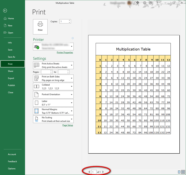
At this point, I would go through and make my Multiplication Table pretty – aka, more readable. Adjust the cell height and width to make each cell square. Add “All Borders” and make the row at the top tall for a big, bold “Merge & Center” title, like “Multiplication Table.”
Finally I would add some color to my factor row and column, plus boldface, wo we can easily see those factors while you look for the product.
From File>Print look at your preview before your print to make sure it is all on one page. Excel is notorious for not printing the way you want it.
I hope you remembered your times tables and understand relative and absolute references now!
