Years ago, I worked at a university, and I was hiring student workers to help with data entry. The highest priority was accuracy. I wanted to create a skills test using an Excel worksheet that looked like our online application page to test their accuracy. In addition to fill in the blanks, several of the items on our application webpage were drop-down menu choices, so did a quick search to see if Excel could do drop-down choices. It could! The feature was called “Data Validation.” Here is a quick lesson.
Set Up a Drop-Down Spreadsheet
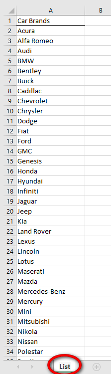
First open a blank Excel spreadsheet and name it “Drop-Down” so we can practice. Now copy this list of car brands and paste it into Cell A1. This will be our list that our data has to match. And thanks to Consumer Reports for this great list. On their page it also shows you who owns which car brands. and you can click on each brand for a link to that website. My list is simply text.
Car Brands
Acura
Alfa Romeo
Audi
BMW
Bentley
Buick
Cadillac
Chevrolet
Chrysler
Dodge
Fiat
Ford
GMC
Genesis
Honda
Hyundai
Infiniti
Jaguar
Jeep
Kia
Land Rover
Lexus
Lincoln
Lotus
Maserati
Mazda
Mercedes-Benz
Mercury
Mini
Mitsubishi
Nikola
Nissan
Polestar
Pontiac
Porsche
Ram
Rivian
Rolls-Royce
Saab
Saturn
Scion
Smart
Subaru
Suzuki
Tesla
Toyota
Volkswagen
Volvo
I put a quick bottom border (Home tab>Font section>Border) under the Car Brands header to differentiate it from the list; always label your data in Excel so when you or someone else opens the spreadsheet, you know immediately what you are seeing.
Create List and Data Worksheets
It is a good practice to keep your list on a separate worksheet so no one accidentally makes changes to the list. Double-click the “Sheet1” worksheet tab at the bottom of your spreadsheet, and rename this worksheet “List.” Click back on your spreadsheet to set the name.
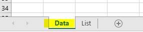
Add a second worksheet by clicking the plus next to the List tab. Name this worksheet “Data.” This is where we will enter the Data. We will check if it is “Valid” against the List. Now you understand the term “Data Validation.” Move the Data tab to the left of the List tab. That way your data entry clerks will open the spreadsheet to the Data page rather than messing up the List.
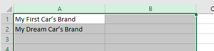
Copy these two lines and paste into Cell A1 (or type into Cells A1 and A2).
My First Car’s Brand
My Dream Car’s Brand
Select Columns A and B and drag so they are twice as wide, about two inches on your screen. I will also add borders around each of the data entry cells in Column B and make them light grey for emphasis. That tells the data entry clerk, “This is where you fill in the blanks.” (Select Range B1:B2, then click the Home tab>Font section>Fill bucket drop-down and select a light grey. Which Range B1:B2 still selected, select Home tab>Font section>Border drop-down>All Borders.)
Now you ready for the Data Validation command.
Data Validation for Data Entry – or – Create the Drop-Down
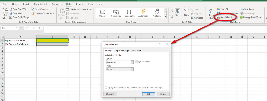
Click on Cell B1, the blank next to “My First Car’s Brand.”
“Data Validation” is on the Data tab. On the Data tab>Data Tools section, click on Data Validation. The icon is two little cells – one with a green checkmark for “yes!” and one with a red “x” for “no!” (There are some drop-down options on the Data Validation icon, but we do not need these.) The Data Validation window will appear.
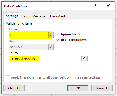
From the Allow drop-down, choose List. Click inside the Source box, then go back to the List tab on the spreadsheet and drag from the first car brand to the last, Range A2:A49, from Acura to Volvo. Do not include the “Car Brands” header. You are showing Excel the range to compare your data to. Only items in this list may be entered. The two checkboxes are checked by default: “Ignore blank” cells and create an “in-cell dropdown.” Click OK.
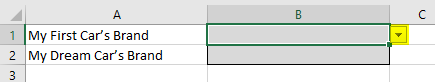
When Excel takes you back to Cell B1, you will notice a small drop-down arrow to the right of the cell. This arrow disappears when another cell is selected and reappears when Cell B1 is selected. (Go ahead, try it!)
Validate Your Data
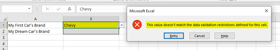
First let’s see if it validates our data with normal text entry. Type “Chevy” in Cell B1 and press Enter.An error message will appear because “Chevy” is not a “valid” entry when Excel compares it to our list. You can either “Retry” or “Cancel” and Excel will delete “Chevy” from Cell B1.
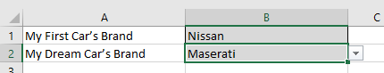
Instead of typing, which is prone to errors and typos, simply click the drop-down arrow next to Cell B1. Our List of car brands will appear. Use the scroll bar to the right of the drop-down list to see all the cars. Select the brand of your very first car by clicking it. Excel will put the brand into Cell B1.
Practice or Copy & Paste
Practice Data Validation in Cell B2 by going back through each step. You can also copy Cell B1 to Cell B2. Select “My Dream Car’s Brand” from Cell B2’s drop-down menu. Which car is your dream car? I like those orange pearl Maserati’s. I’ll take any model, okay?
Save and exit so you will have this sample to look at next time you try drop-down menus… er… I mean Data Validation in Excel.
