I will be devoting three days to this topic. Sorting and filtering information is one of the most efficient uses of Excel, especially for those of us who are not experts at database programs such as MS Access.
When you have a large list of items on your spreadsheet, sometimes you only want to look at certain items, say dogs with curly hair. Let’s make a spreadsheet of dog breeds and traits; you may copy and paste the list below into Excel. (I own a type of Belgian shepherd called a Belgian Tervuren whose story you can see on her website at sahzidog.blogspot.com.)
| Dog Breed | Short | Long | Wired | Curly | Max Size Inches | County of Origin |
| Belgian Shepherd | x | x | x | 26 | Belgium | |
| Boxer | x | 25 | Germany | |||
| Chihuahua | x | x | 9 | Mexico | ||
| Dachshund | x | x | x | 15 | Germany | |
| Flat Coated Retriever | x | 24 | England | |||
| Fox Terrier | x | x | 15 | England | ||
| German Shepherd | x | x | 26 | Germany | ||
| Irish Wolfhound | x | x | 32 | Ireland | ||
| Labrador Retriever | x | 24 | Canada | |||
| Maltese | x | 10 | Greece | |||
| Portuguese Water Dog | x | x | 23 | Portugal | ||
| Shetland Sheepdog | x | 16 | Scotland | |||
| Standard Poodle | x | x | 21 | Germany |
Once we have the table set up, we can either add filters to the headings or format it as a table. Today, we will simply add filters.
Add Filters without Using a Table
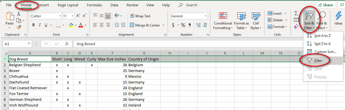
Highlight the row with the headings by clicking on the number next to the row. In our example, it’s Row 1. Then click on the Sort & Filter icon in the Editing section of the Home Ribbon. Click on Filter in the drop down menu. The Filter icon is a funnel or strainer because you are going to be straining out the items you want.
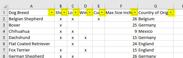
Now a small upside-down triangle will appear in the corner of every cell in the headings. This of this as a tiny version of the funnel to remind you that you can strain out your results.
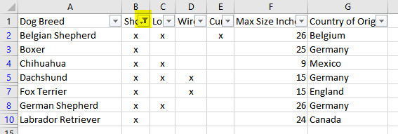
To look at just the short hair dogs, click on the triangle in the “Short” column. When the drop-down filter menu appears, click on the check next to “(Blanks)”. This will deselect or hid any cells below that are blank. In this case, only the cells with an “x” will remain visible. If the cells had x’s and o’s, you could click on “(Select All)” to clear everything, then just click on the one you want and click OK. Now the down triangle will have a funnel next to it to show you that your are filtering that particular column.
Now the down triangle will have a funnel next to it to show you that your are filtering that particular column.
To get all your dogs back, click the filter, and check “Select All” and OK.
Important Tip: DO NOT use the sort function in the drop down menu above for an individual column now. You must either select all your data first, or format the data as a table first. If you sort on your Dog Breed column only right now, your dog breeds will be alphabetical, but the other columns will stay where they are, in other words, the Portuguese Water Dog will suddenly have its origins in Canada.
Now that your spreadsheet is ready, save it, and go to the next two lessons
- Excel: Why should I use “Format as Table” command when my table is already there?
- Excel: Counting with Totals Row in a Table

2 Comments