In the last two lessons, we learned about Filtering and Excel’s Format as Table command. Open up the dog breed spreadsheet we’ve been working on. If you need the data, copy and paste the spreadsheet at the bottom into Excel.
Adding or Counting with =counta()
Let’s say we want to count our short hair dogs. The keyword here is “Count.” We are not totaling something, say adding the inches, instead we are counting the number of dogs. In Excel go to the cell where you want the answer, then type “=”. This creates a formula. The formula we want is =counta() which counts cells that have something in them; it counts anything that is not an empty cell. In our Dog Breed spreadsheet from the previous lessons, it will count the “x” in the columns.
In the column labeled Short, go to an empty cell a few rows below the last dog: Cell B17. Type “=counta” and add an open-parenthesis “(“:
=counta(
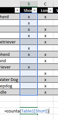
The open parenthesis tells Excel that you are going to give it a range of cells on which to work its magic. Now, drag through the data between the heading “Short” and the last cell of our table, Cell B2 to B14). Do not include your heading! Excel will replace the cell names with a range specific to the table: “Table1[Short].” This shows it is the entire “Short” column in the table. Type close-parenthesis “)” to tell Excel you are finished with the range, then press Enter to “enter” the formula.
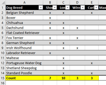
There are seven short hair dogs in our list. Excel also added a total line to our table. Do the same procedure in the Long, Wired, and Curly columns. Copy and Paste do not work quite the same in tables, so just create the =acount() formula in each column.
…or…
You can drag the formula from B17 to the other columns. Click on Cell B17. Notice the little dot in the bottom right of the cell. Hover your mouse over the dot and it will turn into narrow plus-sign called the “drag cursor.” Click and drag through cells C17, D17, and E17. When you release your mouse, Excel will create a “relative” formula in each cell, relative to the column in your table above. Instead of counting the x’s in the “Short” column, the formula in C17 counts the x’s in the “Long” column, and so on.
This is how to manually add the =counta() formula, but let’s learn how to have Excel’s Table Row feature instead.
Add Totals Row
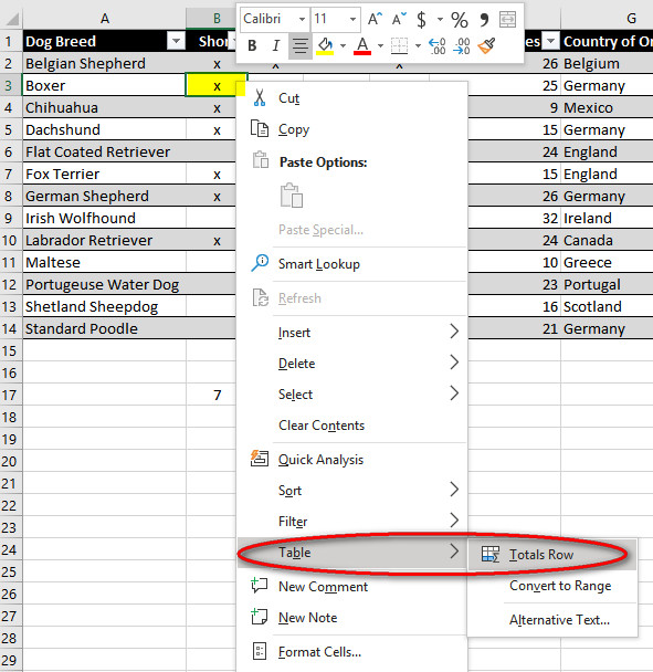 Click in any cell in the table, let’s say on the “x” next to Boxer, although any cell INSIDE the table will do. Right-click and find the Table item in the pop-up list that appears. As you hover over “Table” a new menu pops up. Select “Totals Row” from the list.
Excel will add a Totals Row to your Table. It will add the word “Total” to the lefthand cell. In the bottom right cell, it will either total any numbers or count the items in the righthand column. It has counted our thirteen dogs.
Click on the Totals Row under the “Short” column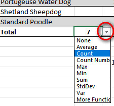 . When you click any cell in the Totals Row, a small drop-down arrow appears next to the cell. Click the drop-down arrow. Notice that you have a choice of formulas. Choose “Count” to count our short-haired dogs.
. When you click any cell in the Totals Row, a small drop-down arrow appears next to the cell. Click the drop-down arrow. Notice that you have a choice of formulas. Choose “Count” to count our short-haired dogs.Do this for each coat-type column.
Whenever I change the Totals Row from a “Sum” or adding numbers, I like to change the word “Total” in Column A to an appropriate word, like “Count.”
Filter Your Count
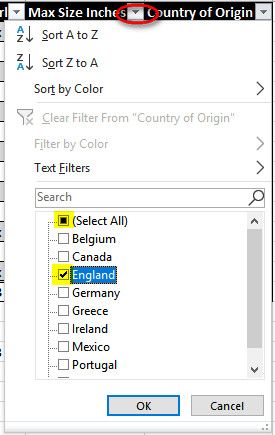
This gives us a count of coat types, but it doesn’t tell us things like how many dogs from England have short hair. Let’s filter out all the dogs except the dogs that originated in England by clicking the filter triangle in the Country of Origin column, click on the check next to Select All to deselect all the countries, then just click the checkbox next to England and OK.
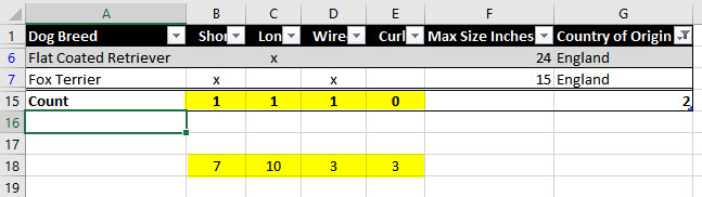
Only two dogs are now visible, and the Totals Row reflects those two dogs.
Take a look at the numbers from our =counta() formulas. They used to be on Row 17, but when we added the Totals Row, Excel dropped them down to Row 18. These formulas are outside your table, so the filter does not change the results. That is one of the powerful reasons to use Tables.
Play with your table for a while until you are comfortable. Before you exit and save, always go back to any filtered results, such as Country of Origin, select the Filter (funnel) and click “Select All.” That way you will not open your list and wonder where your other dogs went.
________________________________________________________
Sample Spreadsheet to Copy & Paste into Excel:
| Dog Breed | Short | Long | Wired | Curly | Max Size Inches | County of Origin |
| Belgian Shepherd | x | x | x | 26 | Belgium | |
| Boxer | x | 25 | Germany | |||
| Chihuahua | x | x | 9 | Mexico | ||
| Dachshund | x | x | x | 15 | Germany | |
| Flat Coated Retriever | x | 24 | England | |||
| Fox Terrier | x | x | 15 | England | ||
| German Shepherd | x | x | 26 | Germany | ||
| Irish Wolfhound | x | x | 32 | Ireland | ||
| Labrador Retriever | x | 24 | Canada | |||
| Maltese | x | 10 | Greece | |||
| Portuguese Water Dog | x | x | 23 | Portugal | ||
| Shetland Sheepdog | x | 16 | Scotland | |||
| Standard Poodle | x | x | 21 | Germany |

2 Comments