In a previous blog, I introduced filtering, but warned you not to use the sort command when you use filtering in your header row (unless you highlight your whole spreadsheet first). Today, I’ll show you the best way to sort your data AFTER you format it as an Excel table.
Most of our data in Excel is viewed as a table whether or not it is formatted that way. When you use the “Format as Table” command, Excel looks at your data differently. Sometimes adding or deleting data in a table can be stormy, but manipulating what is already there is a breeze.
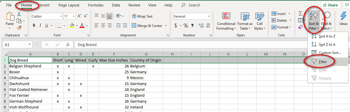
Yesterday, we created a dog breed spreadsheet. If you saved it yesterday, you will need to remove the filters we created. Open the spreadsheet. Remove the filters by following the same steps we used to turn them on. Click on Row 1. From the Home ribbon, Editing section, click on the Sort & Filter icon, then pull down Filter.
Now the little down triangles will disappear, and our spreadsheet looks how it did when we started. You must always remove any filters before doing “Format as Table;” Excel will not perform the command with Filters (try it and see).
If you did not create the dog breed spreadsheet yet, you may copy and paste the data from the bottom of this post; however, I would recommend doing yesterday’s filtering lesson before you proceed.
When your dogs are ready, drag through the whole spreadsheet, starting with the left side of the heading row and going down to the bottom right corner. (Did you know that Standard Poodles came from Germany, not France?)
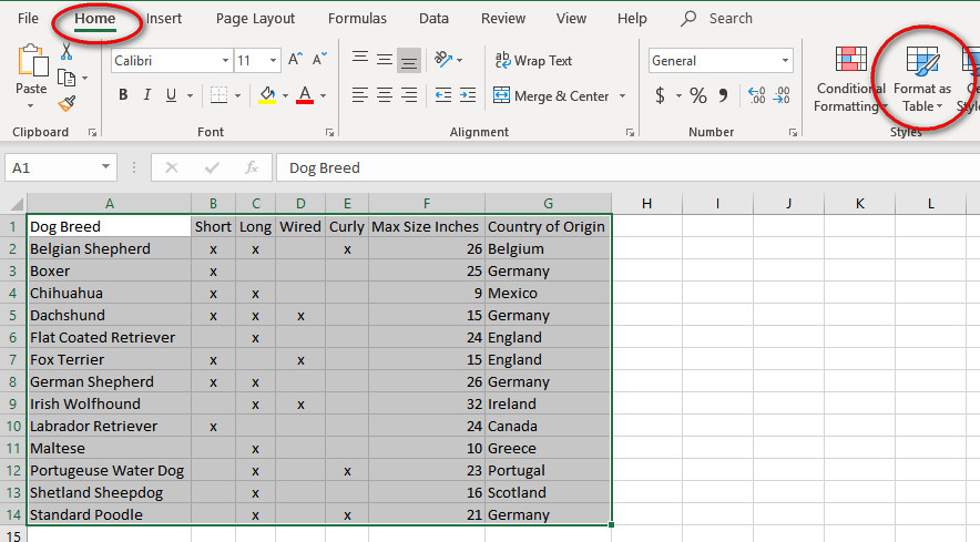
 After you drag through your range of date, on the Home ribbon, Style section, click on the “Format as Table” drop-down arrow.
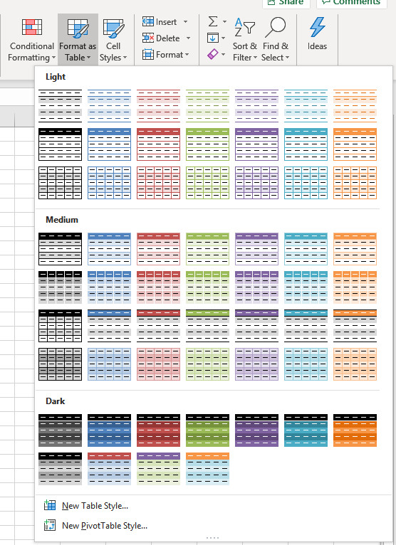
 There are many different colors and formats to choose from – use the one that is easiest on your eyes or your favorite color. We can change it later, so try something daring. After you select a scheme, a window will appear showing your range (the cells you want in your entire table), and asking if your table has headers. Headers means column titles. Ours does, so click OK.
Here’s my newly formatted table:
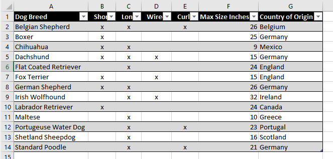
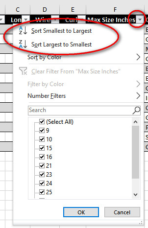 I can now filter the x’s as we did yesterday, but I can also sort. Click on the down triangle in the Dog Breed cell. I can either select certain breeds or sort A to Z or Z to A. Click on the Max Size Inches triangle and I can pick specific heights or sort smallest to largest or largest to smallest. Let’s select only the dog breeds which originated in Germany. Then sort them by size.
 _______________________________________
Here is the spreadsheet you may copy and paste into Excel for this lesson.
| Dog Breed | Short | Long | Wired | Curly | Max Size Inches | County of Origin |
| Belgian Shepherd | x | x | x | 26 | Belgium | |
| Boxer | x | 25 | Germany | |||
| Chihuahua | x | x | 9 | Mexico | ||
| Dachshund | x | x | x | 15 | Germany | |
| Flat Coated Retriever | x | 24 | England | |||
| Fox Terrier | x | x | 15 | England | ||
| German Shepherd | x | x | 26 | Germany | ||
| Irish Wolfhound | x | x | 32 | Ireland | ||
| Labrador Retriever | x | 24 | Canada | |||
| Maltese | x | 10 | Greece | |||
| Portuguese Water Dog | x | x | 23 | Portugal | ||
| Shetland Sheepdog | x | 16 | Scotland | |||
| Standard Poodle | x | x | 21 | Germany |

2 Comments